Recently, in January, I finished the development of the first version of a spectral unmixing function being part of RStoolbox, an R package offering numerous tools for remote sensing analysis written by Benjamin Leutner. The multiple endmember spectral mixture analysis (mesma) function makes it possible to unmix multi- and hyper-spectral imagery by sets of spectral endmember profiles.
For this, a non-negative least squares (NNLS) solver was implemented. NNLS is a statistical approach to fit model parameters to data, assuming that the model parameters are always expressed linearly to those not expressed by the model (unknown parameters) and that the model parameters can never be negative. There are different approaches to solve the NNLS problem. A popular one had been introduced by Lawson & Hanson (1974), which can be considered as fundamental work on practical Least Square Problems solving. It was originally published as FORTRAN code, which is still widely used, e.g. by the R NNLS package or by the Python scipy library. However, compared to newer developing frameworks and languages emerged, the FORTRAN implementation is relatively slow. Thus and to be independent from existing solutions, I wrote a C++ NNLS solver for mesma(), based on a sequential coordinate-wise algorithm (SCA) introduced by Franc et al. (2005). The latter method inherits strong control about the solver’s iteration stopping conditions.

Apart from NNLS, we are planning to add further solver methods (which is why I am currently looking for other practicable unmixing methods).
In this post, I want to demonstrate, how to use the unmixing function RStoolbox::mesma() by giving an example. It can be reproduced on any device running R and having installed the current RStoolbox beta. To do so, execute devtools::install_github(“bleutner/RStoolbox”).
First, we are going to load the Landsat example imagery delivered with RStoolbox:
[code language=”R”]
#if not already done, install RStoolbox beta:
devtools::install_github("bleutner/RStoolbox")
#required caret 6.0-79, which is not on CRAN yet
#load packages
library(raster)
library(RStoolbox)
#load an example dataset
data(lsat)
[/code]
To create some endmember spectra, we simply collect the spectral profiles of “water” and “land” from our imagery. We keep it simple here – instead, you could use spectra from a spectral library.
[code language=”R”]
#make up some endmember spectra: water and land
em_names <- c("water", "land")
pts <- data.frame(class=em_names, cell = c(47916,5294))
em <- lsat[pts$cell]
rownames(em) <- em_names
[/code]
That’s all for the pre-processing! Now you have an image and two endmembers. Note that you need to have at least two endmembers (as we have in this example) to unmix an image. Also, take a look at “em” and “lsat” before continuing: Both have the same spectral resolution (band number), which is a prerequisite. This means that if you want to use data from a spectral library for unmixing, you simply need to resample the data to the same spectral resolution of your imagery to use mesma().
Now, just call mesma(). It returns a probability raster, each layer representing one class of your endmembers, except for the last layer, which gives you the RMSE for each pixel.
[code language=”R”]
#unmix the image for water and land
probs <- mesma(lsat, em, method = "NNLS")
[/code]
Since we decided to develop the NNLS solver from scratch in C++ and not to use existing older FORTRAN implementations, mesma() is quiet fast. It supports parallel processing, if you want to unmix large amounts of data and have multiple CPU cores available. To do so, just create a cluster before calling mesma() using raster::beginCluster() and stop it afterwards using raster::endCluster().
Now, let us look at the output’s:
[code language=”R”]
#take a look
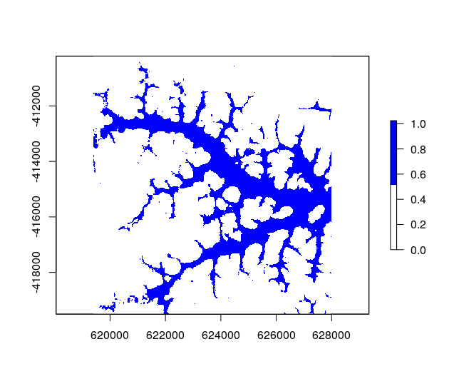
raster::plot(probs$water, col = c("white","blue"))
raster::plot(probs$land, col = c("white","brown"))
[/code]
Here are the probabilities for water…

and here they are for land:

You clearly see, how mesma() could easily differentiate between these two endmembers with only one spectrum per class. If you have ideas or find a problem, please report us via GitHub!
References:
Franc, V., Hlaváč, V., & Navara, M. (2005). Sequential coordinate-wise algorithm for the non-negative least squares problem. In: International Conference on Computer Analysis of Images and Patterns (pp. 407-414). Berlin, Heidelberg.
Lawson, C. L., & Hanson, R. J. (1974). Solving least squares problems (Vol. 15). Siam.

